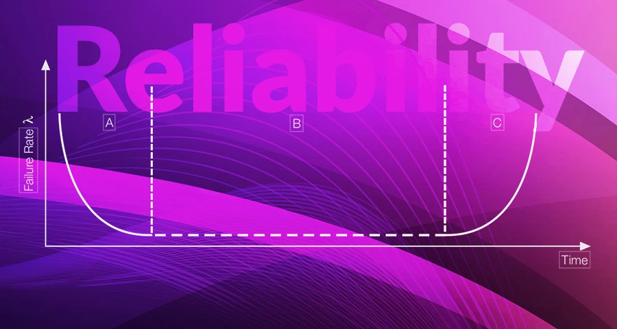
Failure Rate λ
Failure rate is defined as the percentage of units failing per unit time. This varies throughout the
life of the equipment and if λ is plotted against time, a characteristic bathtub curve (below) is
obtained for most electronic equipment.

The curve has three regions, A - Infant mortality, B - Useful life, C - Wear out.
In region A, poor workmanship and substandard components cause failures. This period is usually over within the first few tens of hours and burn-in is normally employed to prevent these failures occurring in the field. Burn-in does not entirely stop the failures occurring but is designed to ensure that they happen within the manufacturing location rather than at the customer’s premises or in the field.
In region B the failure rate is approximately constant and it is only for this region that the following analysis applies.
In region C, components begin to fail through reaching end of life rather than by random failures. Electrolytic capacitors dry out, fan bearings seize up, switch mechanisms wear out and so on. Well implemented preventative maintenance can delay the onset of this region.
Reliability
Reliability is defined as the probability that a piece of equipment operating under specified conditions will perform satisfactorily for a given period of time. Probability is involved since it is impossible to predict the behavior with absolute certainty. The criterion for satisfactory performance must be defined as well as the operating conditions such as input, output, temperature, load etc.
MTBF – Mean Time Between Failures
MTTF – Mean Time To Failure
MTBF applies to equipment that is going to be repaired and returned to service, MTTF to parts that will be thrown away on failing. MTBF is the inverse of the failure rate and is often misunderstood. It is often assumed that the MTBF figure indicates a minimum guaranteed time between failures. This assumption is incorrect, and for this reason the use of failure rate rather than MTBF is recommended.
The mathematics are expressed as follows:

This shows that for a constant failure rate, plotting reliability ‘R(t)’ against time ‘t’ gives a negative exponential curve. When t/m = 1, i.e. after a time ‘t’, numerically equal to the MTBF 1.0 figure ‘m’, then

This equation can be interpreted in a number of ways:

a) If a large number of units are considered,
only 37% of them will survive for as long as the MTBF figure.
b) For a single unit, the probability that it will work for as long as its MTBF figure is only 37%.
c) The unit will work for as long as its MTBF figure with a 37% Confidence Level.
To put these numbers into context, consider a power supply with an MTBF of 500,000 hrs (or a failure rate of 0.002 failures per 1000 hrs), or as the advertisers would put it, an MTBF figure of 57 years. Using the above equation, R(t) for 26,280 hours (three years) is approximately 0.95 and if such a unit is used 24 hours a day for three years the probability of it surviving is 95%. The same calculation for a ten year period will give an R(t) of 84%. If 700 units are used, on average 0.2%/1000hrs will fail, or approximately one per month.

There is no direct connection or correlation between service life and failure rate. It is perfectly possible to design a very reliable product with a short life. A typical example is a missile, which has to be very very reliable (MTBF of several million hours), but its service life is only around 4 minutes (0.06hrs). 25-year-old humans have an MTBF of about 800 years,(failure rate of 0.1% per year), but not many have a comparable service life. If something has a long MTBF, it does not necessarily have a long service life.

Gary Bocock
Gary is a seasoned electronics engineer and a Member of the Institution of Engineering and Technology (MIET). With over three decades of experience in the power supply industry, he has held design, development, applications and management roles. For over 25 years, Gary has been a key figure at XP Power, where he has held various engineering and management positions, ultimately rising to the role of Technical Director.